Moment of Inertia Lab
Author: Jacob Hoffner
Lab Partners: Zach Christoff and Alyssa Jordan
Date: February 2016
Lab Partners: Zach Christoff and Alyssa Jordan
Date: February 2016
Purpose
To determine the Moment of Inertia of an object.
Theory
|
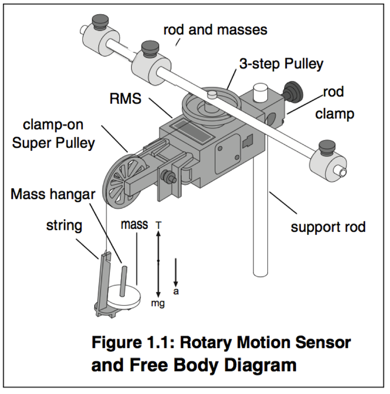
The Moment of Inertia on an object is the quantity of that object that expresses the tendency to resist angular acceleration. In this lab, we are deriving a equation that will find this Moment of Inertia. We are to find the Moment of Inertia of a thin rod with three point masses attached; the rod is spinning on a point in the center of mass, or the center of the rod.
The rod and its point masses will be acceleration and an angular rate due to the weight of a hanging mass over a pulley. The theory of the lab is that the Moment of Inertia calculated from the equations we know will be the same as the Moment of Inertia measured from the data collected from the rod and its point masses. An equation derived from what we know before conducting the experiment should be able to give us an answer that should be the same as the answer found after conducting the experiment. |
|
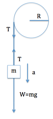
Part 1In order to derive an equation, we must sum the forces that are acting upon the rod. In the Free Body Diagram shown on the right, we can see the different forces acting upon the rod, which ultimately applies the rod’s angular acceleration.
First, we must sum the forces acting upon the hanging mass, string, and pulley. We discover that tension and weight are these forces, and we derive the equation for tension. Meanwhile, we know that we are deriving an equation for the Moment of Inertia. We know that torque equals the Moment of Inertia multiplied by angular acceleration; we may derive this equation for Moment of Inertia. Since we also know that torque equals the radius of the pulley multiplied by the perpendicular force acting causing the torque, which is tension, we may substitute "RT" for torque. We now go back to the equation derived for tension, and substitute this equation in for the tension in the new Moment of Inertia equation. Knowing that tangential acceleration equals the Radius of the pulley multiplied by the angular acceleration, we may now fully derive an equation for the Moment of Inertia. |
|
|
Step 1

|
Sub-Step 1

Sub-Step 2

|
Step 2

|
Part 2Above we have just derived an equation for the calculated Moment of Inertia. In order to prove this theory, we must now derive an equation and solve it using measured values from the lab.
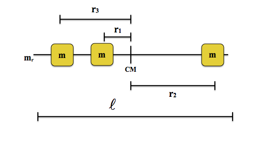
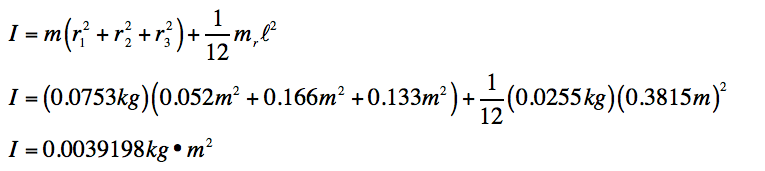
Starting with the components of the lab, we know that the rod and the three point masses all have a Moment of Inertia. Therefore, the measured Moment of Inertia equation will be the sum of these four individual Moments of Inertia, or "I". As "I" equals the mass of the object multiplied by its squared radius, the rod, due to its centralized center of mass, has a distinct Moment of Inertia. Each point mass has the same mass, and their "r"-value is the distance from their center of mass to the rod's center of mass. The cursive "l" is the length of the rod. The rod has a different mass from the point masses. This equation is then derived and simplified for I (Moment of Inertia). |

|
Experimental Technique
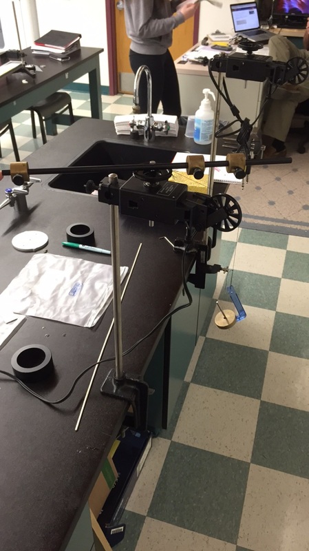
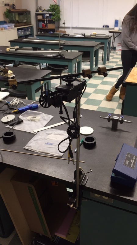
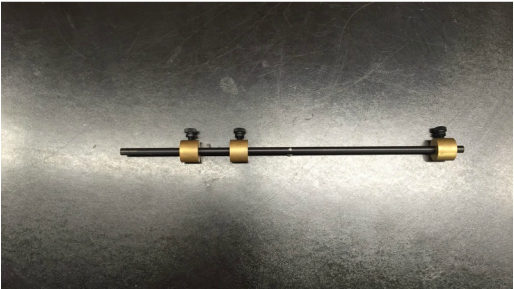
eIn order to begin this lab, we first had to pick the type of object we wanted find its Moment of Inertia. I chose the rod. Three masses were placed on the rod; two on one side of the center of mass, and one on the other side. The masses were balanced evenly on each side of the rod. The rod and masses were placed on the side for now. A C-clamp was then anchored to a table-top, and a long pole was attached vertically. A pulley sensor (for lack of better words) was clamped on the top of the pole. This sensor measures the angular acceleration by plugging the data it finds into an Angular Velocity vs. Time graph on DataStudio.
The rod I had placed to the side is now screwed into the top of the pulley sensor. On the side of the pulley sensor, a separate pulley is anchored on in the opposite orientation. A string is looped around the pulley sensor's "pulley" and then fed over the pulley just attached. At the end of the string, a mass is attached.
We are to measure the angular acceleration of the rod and masses. In order to do so, the mass is released, which pulls the string wrapped around the pulley sensor. The angular acceleration of the rod and masses attached to that pulley sensor is measured through the sensor into DataStudio in the Angular Velocity vs. Time graph.
This measured angular acceleration is later used in the measured Moment of Inertia equation in order to compare with the calculated Moment of Inertia found. The measured Moment of Inertia will then be found using the derived equation, and it will be compared with the calculated Moment of Inertia found with another derived equation. Percent Difference will be calculated to see how close the measured and calculated quantities came out to be.
|
|
Data
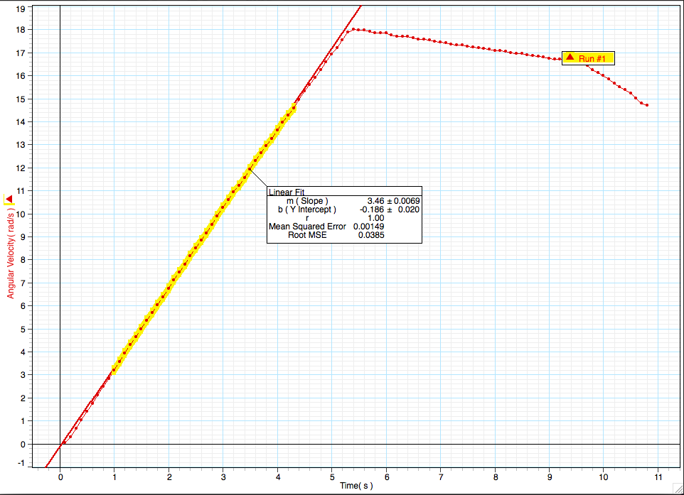
Below is the Angular Velocity vs. Time graph, which indicates the angular acceleration due to the slope of the line.
Below is the information used to solve for the Moment of Inertia, as well as the Calculated and Measured Moment of Inertia, and Percent Difference.
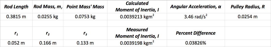
The Hanging Mass that caused the overall angular acceleration was 0.055 kg.
R1, R2, and R3 represent the distance the point masses were from the center of the rod, or the rod's center of mass.
Due to high accuracy between the calculated and measured Moments of Inertia, these values were rounded to five significant figures.
R1, R2, and R3 represent the distance the point masses were from the center of the rod, or the rod's center of mass.
Due to high accuracy between the calculated and measured Moments of Inertia, these values were rounded to five significant figures.
Analysis
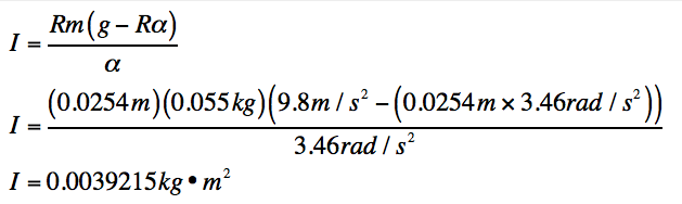
Below are the Sample Calculations (or all of the calculations) for this lab, and are as follows: Calculated Moment of Inertia, Measured Moment of Inertia, and the Percent Difference between the two.
Calculated Moment of Inertia
Measured Moment of Inertia
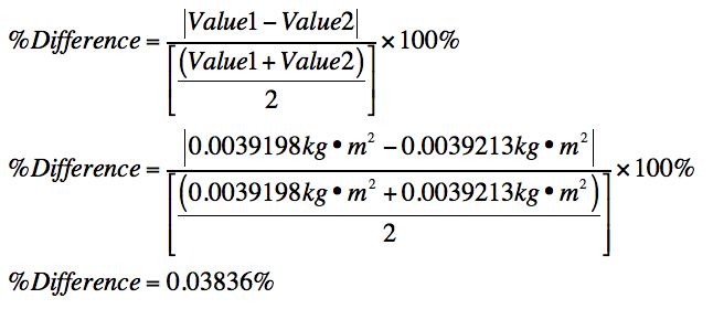
Percent Difference
Conclusion
This lab proved to be very successful. By the end of the lab, the theory was proven. Equations were derived for Moment of Inertia for the measured and calculated values. By gathering careful measurements and solving various variables, we were able to solve for the Moment of Inertia of a rod and point masses. Between the calculated and measured percent differences, there was only about a 0.04% difference; the two values came out very accurately. Because of this very small difference, I had to expand the values from three to five significant figures in order to contrast them. Errors in this lab could in Parallax Error, as measuring the radii of objects can be slightly off when trying to align the measuring tool with an objects center of mass. The string that was wound, causing the angular acceleration of the rod and point masses, could have been bunched up, creating a larger radius of the overall pulley and ultimate error in the lab. There could have been minuscule friction and air resistance, causing a slight error in measurements. Overall, this lab was extremely successful, and extremely accurate.
References
Giancoli, Douglas C. "Angular Quantities." Physics for Scientists & Engineers with Modern Physics. 4th ed. Upper Saddle River, NJ: Prentice Hall, 2000. Print.
Bowman, D. (n.d.). Lahs Physics. Retrieved October 1, 2015, from http://lahsphysics.weebly.com/
Bowman, D. (2015, October 1). Chapter 10: Angular Quantities. Lecture presented at Physics, Lehighton.
Bowman, D. (n.d.). Lahs Physics. Retrieved October 1, 2015, from http://lahsphysics.weebly.com/
Bowman, D. (2015, October 1). Chapter 10: Angular Quantities. Lecture presented at Physics, Lehighton.
