Atwood's Device
Author: Jacob Hoffner
Lab Partners: Andrea Schaefer and Connor Frey
Date: November 2015
Lab Partners: Andrea Schaefer and Connor Frey
Date: November 2015
Purpose
Forces will be identified and studied using Atwood's Device. Acceleration will be predicted by summing the forces, F=ma, of two different objects and deriving an equation in order to investigate the correlation between the predicted acceleration and the measured acceleration using Newton's 2nd Law of Motion.
Theory
George Atwood was an English mathematician who was born in 1745 and was a very popular lecturer at Cambridge through the 1770's. He is best known for a work, A Treatise on the Rectilinear Motion and Rotation of Bodies, which is a textbook describing the mechanics of Newton's laws through impact and simple harmonic motion. The book describes Atwood's Device, which was created in order to demonstrate the laws of uniformly accelerated motion due to gravity. The device first appeared in France in 1780, and since then copies had been sent to Spain, where it latter was introduced to the rest of the world. Atwood's Device is used to present Newton's Second Law of Motion through summing the forces, F=ma.
|
In order to derive an equation to solve for acceleration, we must first set up an equation to find acceleration. To start, we observe the Free Body Diagram (FBD) that is to the right. Acceleration occurs due to Object 2 in the FBD having a bigger mass.We are to find the acceleration in the positive direction.
First, we must always sum the forces: F=ma. Since we have two masses, the forces are summed individually for each, F1 and F2.
|
Free Body Diagram (FBD)
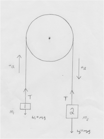
T=T W2>W1
W2>T (Weight 2 Vector Arrow > Tension Vector Arrow) |


We already know that T=T, since Tension is equal on both Object 1 and Object 2. Because of this, using the Transitive Property, the two expressions T equals can now be set equal to each other.

Now that both of Tension's solutions are set equal to each other, we can now derive for acceleration, a. In theory, we discover that acceleration equals: g[(m2-m1)/(m1-m2)].
Experimental Technique
|
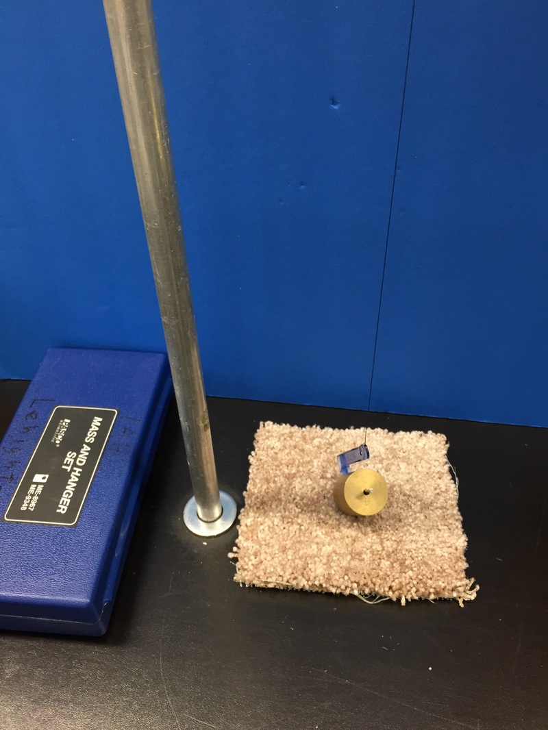
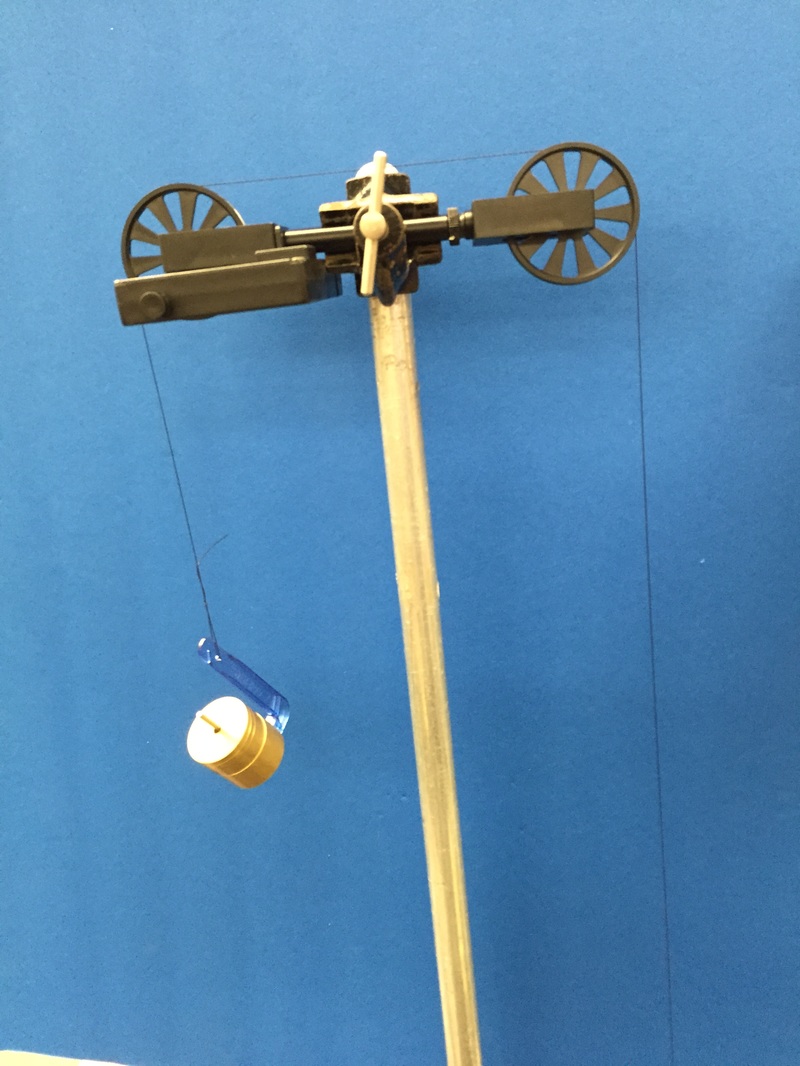
In order to receive different three different accelerations for Atwood's Device, we used three different sets of masses for Object 1 and Object 2. While keeping into account the mass of the mass of the mass-holder, we summed up the total grams on each mass-holder plus the grams of the masses. Error was attempted to be reduced by increasing the difference in mass between Object 1 and Object 2 per run. By holding the heavier Object at the top of Atwood's Device, we let it go and measure acceleration of that Object falling by using a photo-gate connected to Atwood's Device. By doing this three times, the photo-gate records the data onto a graph on DataStudio. By taking the slope of the Velocity vs. Time graph, we can discover the acceleration of the falling Object (Object 2). We then calculate acceleration for the three runs by using the equation derived in theory. By comparing the measured acceleration with the calculated acceleration using percent difference, we can determine the accuracy of our theory.
|
|
Data
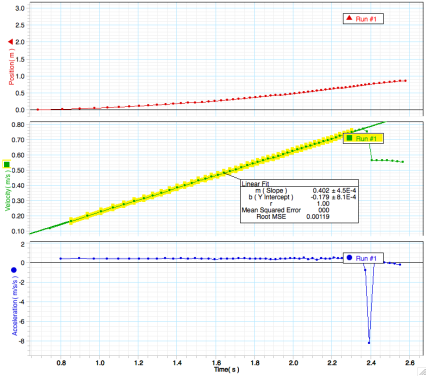
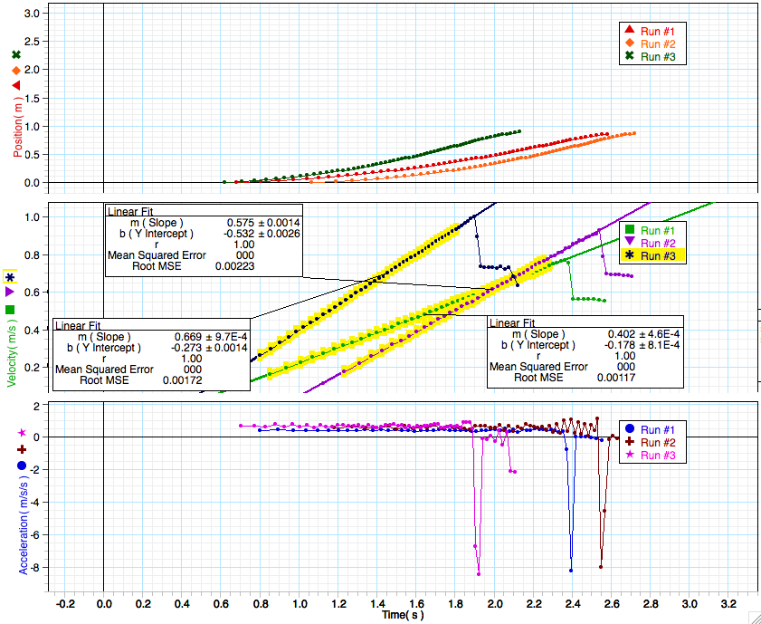
Below are the graphs used to find acceleration. The Velocity vs. Time graph (center graph) is presented below so the slope can be used to find acceleration. The graph to the left indicates the slope of Run 1 as an example, which yields 0.402 m/s/s. The graph to the left indicates all three slopes of all Runs 1-3.
|
|
Below are the masses that were used in each run above, as well as the measured and calculated accelerations and percent difference. Each row indicates the results of one run above.
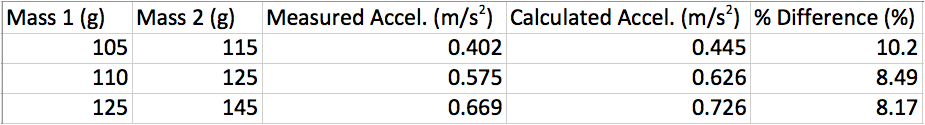
Average Percent Difference: 8.95%
Analysis
The following sample calculations exemplify the derived acceleration equation and percent difference.
|
Acceleration

|
Percent Difference

|
Conclusion
The main purpose of this lab was to discover if the equation derived to find acceleration yielded an answer close to the acceleration measured. The predicted and measured accelerations compare quite closely to one another; considering that the average percent difference was 8.95%, the overall error in acceleration was not substantial. Parallax error in release the Objects in a straight line would have been the biggest error, however it would have been picayune, since acceleration was measured by the photo-gate, which eliminates most human error. However, human error could have been a major contributor to the differences in the objects' accelerations. The release of the masses could have resulted in string wobble, especially when the masses hit the table, which could have yielded a line that was not perfectly straight on the graph, resulting in slight acceleration inaccuracy. All in all, the predicted accelerations proved quite reliable to the measured accelerations. In order to reduce error, we increased the difference in masses of the two Objects in each run. However, this method resulted in an increase in error. The antipode in the order or runs, however, would have yielded a reduction in error (in other words, starting from Run 3 to Run 1 reduced error). Overall, we have learned that having a smaller difference in mass between the two Objects yields a lower percent difference, thus a reduction in error. Thence, we have discovered that our theory is proven correct; due to the low yield in percent difference, it can be stated that the equation derived for acceleration can be used to accurately calculate acceleration in relation to Newton's 2nd Law of Motion.
References
George Atwood. (2005, February 1). Retrieved November 14, 2015, from http://www-history.mcs.st-andrews.ac.uk/Biographies/Atwood.html
Giancoli, D. (1998). Chapter 3: Kinematics in Two Dimensions; Vectors. InPhysics: Principles with applications (5th ed., p. 1096). Upper Saddle River, N.J., New Jersey: Prentice Hall.
Bowman, D. (2015, October 1). Chapter 3: Kinematics in Two Dimensions; Vectors. Lecture presented at Physics, Lehighton.
Bowman, D. (n.d.). Lahs Physics. Retrieved October 1, 2015, from http://lahsphysics.weebly.com/
